Steps 1-6
- Load the R packages we will use.
- Read the data in the files,
drug_cos.csv,health_cos.csvinto R and assign to the variablesdrug_cosandhealth_cos, respectively.
drug_cos <- read.csv("http://estanny.com/static/week6/drug_cos.csv")

health_cos <- read_csv("http://estanny.com/static/week6/health_cos.csv")
- Use
glimpseto get a glimpse of the data
drug_cos %>% glimpse()
Rows: 104
Columns: 9
$ ticker       <chr> "ZTS", "ZTS", "ZTS", "ZTS", "ZTS", "ZTS", "Z...
$ name         <chr> "Zoetis Inc", "Zoetis Inc", "Zoetis Inc", "Z...
$ location     <chr> "New Jersey; U.S.A", "New Jersey; U.S.A", "N...
$ ebitdamargin <dbl> 0.149, 0.217, 0.222, 0.238, 0.182, 0.335, 0....
$ grossmargin  <dbl> 0.610, 0.640, 0.634, 0.641, 0.635, 0.659, 0....
$ netmargin    <dbl> 0.058, 0.101, 0.111, 0.122, 0.071, 0.168, 0....
$ ros          <dbl> 0.101, 0.171, 0.176, 0.195, 0.140, 0.286, 0....
$ roe          <dbl> 0.069, 0.113, 0.612, 0.465, 0.285, 0.587, 0....
$ year         <int> 2011, 2012, 2013, 2014, 2015, 2016, 2017, 20...
health_cos %>% glimpse()
Rows: 464
Columns: 11
$ ticker      <chr> "ZTS", "ZTS", "ZTS", "ZTS", "ZTS", "ZTS", "ZT...
$ name        <chr> "Zoetis Inc", "Zoetis Inc", "Zoetis Inc", "Zo...
$ revenue     <dbl> 4233000000, 4336000000, 4561000000, 478500000...
$ gp          <dbl> 2581000000, 2773000000, 2892000000, 306800000...
$ rnd         <dbl> 427000000, 409000000, 399000000, 396000000, 3...
$ netincome   <dbl> 245000000, 436000000, 504000000, 583000000, 3...
$ assets      <dbl> 5711000000, 6262000000, 6558000000, 658800000...
$ liabilities <dbl> 1975000000, 2221000000, 5596000000, 525100000...
$ marketcap   <dbl> NA, NA, 16345223371, 21572007994, 23860348635...
$ year        <dbl> 2011, 2012, 2013, 2014, 2015, 2016, 2017, 201...
$ industry <chr> "Drug Manufacturers - Specialty & Generic", "...- Which variables are the same in both data sets
names_drug <- drug_cos %>% names()
names_health <- health_cos %>% names()
intersect(names_drug, names_health)
[1] "ticker" "name" "year" - Select subset of variables to work with
For
drug_cosselect (in this order):ticker,year,grossmargin-Extract observations for 2018
-Assign output to
drug_subset
-For health.cos select (in this order): ticker , year , revenue , gp , industry
-Extract observations for 2018
-Assign output to health_subset
- Keep all the rows and columns
drug_subsetjoin with columns inhealth_subset
drug_subset %>% left_join(health_subset)
   ticker year grossmargin     revenue          gp
1     ZTS 2018       0.672  5825000000  3914000000
2    PRGO 2018       0.387  4731700000  1831500000
3     PFE 2018       0.790 53647000000 42399000000
4     MYL 2018       0.350 11433900000  4001600000
5     MRK 2018       0.681 42294000000 28785000000
6     LLY 2018       0.738 24555700000 18125700000
7     JNJ 2018       0.668 81581000000 54490000000
8    GILD 2018       0.781 22127000000 17274000000
9     BMY 2018       0.710 22561000000 16014000000
10   BIIB 2018       0.865 13452900000 11636600000
11   AMGN 2018       0.827 23747000000 19646000000
12    AGN 2018       0.861 15787400000 13596000000
13   ABBV 2018       0.764 32753000000 25035000000
                                   industry
1  Drug Manufacturers - Specialty & Generic
2  Drug Manufacturers - Specialty & Generic
3              Drug Manufacturers - General
4  Drug Manufacturers - Specialty & Generic
5              Drug Manufacturers - General
6              Drug Manufacturers - General
7              Drug Manufacturers - General
8              Drug Manufacturers - General
9              Drug Manufacturers - General
10             Drug Manufacturers - General
11             Drug Manufacturers - General
12             Drug Manufacturers - General
13             Drug Manufacturers - General
Question: join_ticker
*Start with drug_cos
Extract observations for the ticker MYL from drug_cos Assign output to the variable drug_cos_subset
drug_cos_subset <- drug_cos %>%
  filter(ticker == "MYL")
*Display drug_cos_subset
drug_cos_subset
  ticker     name       location ebitdamargin grossmargin netmargin
1    MYL Mylan NV United Kingdom        0.245       0.418     0.088
2    MYL Mylan NV United Kingdom        0.244       0.428     0.094
3    MYL Mylan NV United Kingdom        0.228       0.440     0.090
4    MYL Mylan NV United Kingdom        0.242       0.457     0.120
5    MYL Mylan NV United Kingdom        0.243       0.447     0.090
6    MYL Mylan NV United Kingdom        0.190       0.424     0.043
7    MYL Mylan NV United Kingdom        0.272       0.402     0.058
8    MYL Mylan NV United Kingdom        0.258       0.350     0.031
    ros   roe year
1 0.161 0.146 2011
2 0.163 0.184 2012
3 0.153 0.209 2013
4 0.169 0.283 2014
5 0.133 0.089 2015
6 0.052 0.044 2016
7 0.121 0.054 2017
8 0.074 0.028 2018- Use left_join to combine the rows and columns of
drug_cos_subsetwith the columns ofhealth_cos
*Assign the output to combo_df
combo_df <- drug_cos_subset %>%
  left_join(health_cos)
*Display combo_df
combo_df
  ticker     name       location ebitdamargin grossmargin netmargin
1    MYL Mylan NV United Kingdom        0.245       0.418     0.088
2    MYL Mylan NV United Kingdom        0.244       0.428     0.094
3    MYL Mylan NV United Kingdom        0.228       0.440     0.090
4    MYL Mylan NV United Kingdom        0.242       0.457     0.120
5    MYL Mylan NV United Kingdom        0.243       0.447     0.090
6    MYL Mylan NV United Kingdom        0.190       0.424     0.043
7    MYL Mylan NV United Kingdom        0.272       0.402     0.058
8    MYL Mylan NV United Kingdom        0.258       0.350     0.031
    ros   roe year     revenue         gp       rnd netincome
1 0.161 0.146 2011  6129825000 2563364000 294728000 536810000
2 0.163 0.184 2012  6796100000 2908300000 401300000 640900000
3 0.153 0.209 2013  6909100000 3040300000 507800000 623700000
4 0.169 0.283 2014  7719600000 3528000000 581800000 929400000
5 0.133 0.089 2015  9429300000 4216100000 671900000 847600000
6 0.052 0.044 2016 11076900000 4697000000 826800000 480000000
7 0.121 0.054 2017 11907700000 4783100000 783300000 696000000
8 0.074 0.028 2018 11433900000 4001600000 704500000 352500000
       assets liabilities   marketcap
1 11598143000  8093361000  9152949366
2 11931897000  8576069000 11186639345
3 15294800000 12334900000 16615987073
4 15820500000 12544500000 21097801310
5 22267700000 12501900000 26588761155
6 34726200000 23608600000 20414265402
7 35806300000 22498700000 22696620826
8 32734900000 20567800000 14128302853
                                  industry
1 Drug Manufacturers - Specialty & Generic
2 Drug Manufacturers - Specialty & Generic
3 Drug Manufacturers - Specialty & Generic
4 Drug Manufacturers - Specialty & Generic
5 Drug Manufacturers - Specialty & Generic
6 Drug Manufacturers - Specialty & Generic
7 Drug Manufacturers - Specialty & Generic
8 Drug Manufacturers - Specialty & Generic- Note: the variables
ticker,name,location, andindustryare the same for all the observations
*Assign the company name to co_name
co_name <- combo_df %>%
  distinct(name) %>%
  pull()
*Assign the company location to co_location
co_location <- combo_df  %>%
  distinct(location) %>%
  pull()
*Assign the industry to co_industry group
co_industry <- combo_df %>%
  distinct(industry) %>%
  pull()
Put the r inline commands used in the blanks below. When you knit the document the results of the commands will be displayed in your text.
The company Mylan NV is located in United Kingdom and is a member of the drug manufacturers industry group.
*Start with combo_df
*Select variables (in this order): year, grossmargin, netmargin, revenue, gp, netincome
*Assign the output to combo_df_subset
combo_df_subset <- combo_df %>%
  select(year, grossmargin, netmargin,
  revenue, gp, netincome)
*Display combo_df_subset
combo_df_subset
  year grossmargin netmargin     revenue         gp netincome
1 2011       0.418     0.088  6129825000 2563364000 536810000
2 2012       0.428     0.094  6796100000 2908300000 640900000
3 2013       0.440     0.090  6909100000 3040300000 623700000
4 2014       0.457     0.120  7719600000 3528000000 929400000
5 2015       0.447     0.090  9429300000 4216100000 847600000
6 2016       0.424     0.043 11076900000 4697000000 480000000
7 2017       0.402     0.058 11907700000 4783100000 696000000
8 2018       0.350     0.031 11433900000 4001600000 352500000
*Create the variable grossmargin_check to compare with the variable grossmargin. They should be equal. - grossmargin_check = gp / revenue
*Create the variable close_enough to check that the absolute value of the difference between grossmargin_check and grossmargin is less than 0.001.
combo_df_subset %>%
  mutate(grossmargin_check = gp / revenue,
  close_enough = abs(grossmargin_check - grossmargin) < 0.001)
  year grossmargin netmargin     revenue         gp netincome
1 2011       0.418     0.088  6129825000 2563364000 536810000
2 2012       0.428     0.094  6796100000 2908300000 640900000
3 2013       0.440     0.090  6909100000 3040300000 623700000
4 2014       0.457     0.120  7719600000 3528000000 929400000
5 2015       0.447     0.090  9429300000 4216100000 847600000
6 2016       0.424     0.043 11076900000 4697000000 480000000
7 2017       0.402     0.058 11907700000 4783100000 696000000
8 2018       0.350     0.031 11433900000 4001600000 352500000
  grossmargin_check close_enough
1         0.4181790         TRUE
2         0.4279366         TRUE
3         0.4400428         TRUE
4         0.4570185         TRUE
5         0.4471276         TRUE
6         0.4240356         TRUE
7         0.4016813         TRUE
8         0.3499768         TRUE
*Create the variable netmargin_check to compare with the variable netmargin. They should be equal.
*Create the variable close_enough to check that the absolute value of the difference between netmargin_check and netmargin is less than 0.001
combo_df_subset %>%
  mutate(netmargin_check = netincome / revenue,
  close_enough = abs(netmargin_check - netmargin) < 0.001)
  year grossmargin netmargin     revenue         gp netincome
1 2011       0.418     0.088  6129825000 2563364000 536810000
2 2012       0.428     0.094  6796100000 2908300000 640900000
3 2013       0.440     0.090  6909100000 3040300000 623700000
4 2014       0.457     0.120  7719600000 3528000000 929400000
5 2015       0.447     0.090  9429300000 4216100000 847600000
6 2016       0.424     0.043 11076900000 4697000000 480000000
7 2017       0.402     0.058 11907700000 4783100000 696000000
8 2018       0.350     0.031 11433900000 4001600000 352500000
  netmargin_check close_enough
1      0.08757346         TRUE
2      0.09430409         TRUE
3      0.09027225         TRUE
4      0.12039484         TRUE
5      0.08989002         TRUE
6      0.04333342         TRUE
7      0.05844957         TRUE
8      0.03082938         TRUE
Question: summarize_industry
Fill in the blanks
Put the command you use in the Rchunks in the Rmd file for this quiz
Use the health_cos data
For each industry calculate mean_grossmargin_percent = mean(gp / revenue) * 100 median_grossmargin_percent = median(gp / revenue) * 100 min_grossmargin_percent = min(gp / revenue) * 100 max_grossmargin_percent = max(gp / revenue) * 100
health_cos %>%
  group_by(industry) %>%
  summarize(mean_grossmargin_percent = mean(gp / revenue) * 100,
            median_grossmargin_percent = median(gp / revenue) * 100,
            min_grossmargin_percent = min(gp / revenue) * 100,
            max_grossmargin_percent = max(gp / revenue) * 100
)
# A tibble: 9 x 5
  industry mean_grossmargi~ median_grossmar~ min_grossmargin~
* <chr>               <dbl>            <dbl>            <dbl>
1 Biotech~             92.5            92.7             81.7
2 Diagnos~             50.5            52.7             28.0
3 Drug Ma~             75.4            76.4             36.8
4 Drug Ma~             47.9            42.6             34.3
5 Healthc~             20.5            19.6             10.0
6 Medical~             55.9            37.4             28.1
7 Medical~             70.8            72.0             53.2
8 Medical~             10.4             5.38             2.49
9 Medical~             53.9            52.8             40.5
# ... with 1 more variable: max_grossmargin_percent <dbl>- mean_grossmargin_percent for the industry Medical Devices is Answer 70.8%
- median_grossmargin_percent for the industry Medical Devices is Answer 72.0%
- min_grossmargin_percent for the industry Medical Devices is Answer 53.2%
- max_grossmargin_percent for the industry Medical Devices is Answer 84.7%
Question: inline_Ticker
Fill in the blanks
Use the health_cos data
Extract observations for the ticker BMY from
health_cosand assign to the variable health_cos_subset
health_cos_subset  <- health_cos  %>%
   filter(ticker == "BMY")
- Display
health_cos_subset
health_cos_subset
# A tibble: 8 x 11
  ticker name  revenue      gp    rnd netincome  assets liabilities
  <chr>  <chr>   <dbl>   <dbl>  <dbl>     <dbl>   <dbl>       <dbl>
1 BMY    Bris~ 2.12e10 1.56e10 3.84e9    3.71e9 3.30e10 17103000000
2 BMY    Bris~ 1.76e10 1.30e10 3.90e9    1.96e9 3.59e10 22259000000
3 BMY    Bris~ 1.64e10 1.18e10 3.73e9    2.56e9 3.86e10 23356000000
4 BMY    Bris~ 1.59e10 1.19e10 4.53e9    2.00e9 3.37e10 18766000000
5 BMY    Bris~ 1.66e10 1.27e10 5.92e9    1.56e9 3.17e10 17324000000
6 BMY    Bris~ 1.94e10 1.45e10 5.01e9    4.46e9 3.37e10 17360000000
7 BMY    Bris~ 2.08e10 1.47e10 6.48e9    1.01e9 3.36e10 21704000000
8 BMY    Bris~ 2.26e10 1.60e10 6.34e9    4.92e9 3.50e10 20859000000
# ... with 3 more variables: marketcap <dbl>, year <dbl>,
#   industry <chr>
In the console, type
?distinct. Go to the help pane to see what distinct doesIn the console, type
?pull. Go to the help pane to see what pull does
Run the code below
health_cos_subset  %>%
  distinct(name) %>%
  pull(name)
[1] "Bristol Myers Squibb Co"- Assign the output to co_name
co_name <- health_cos_subset  %>%
  distinct(name) %>%
  pull(name)
You can take output from your code and include it in your text.
- The name of the company with ticker BMY is
Bristol Myers Squibb Co*
In following chuck
- Assign the company’s industry group to the variable
co_industry
co_industry  <- health_cos_subset %>%
  distinct(industry) %>%
  pull()
This is outside the Rchunck. Put the r inline commands used in the blanks below. When you knit the document the results of the commands will be displayed in your text.
The company Bristol Myers Squibb Cois a member of the Drug Manufacturers - General group.
- Steps 7-11
- Prepare the data for the plots
-start with health_cos THEN -group_by industry THEN -calculate the median research and development expenditure by industry -assign the output to df
- Use
glimpseto glimpse the data for the plots.
df %>% glimpse()
Rows: 9
Columns: 2
$ industry    <chr> "Biotechnology", "Diagnostics & Research", "D...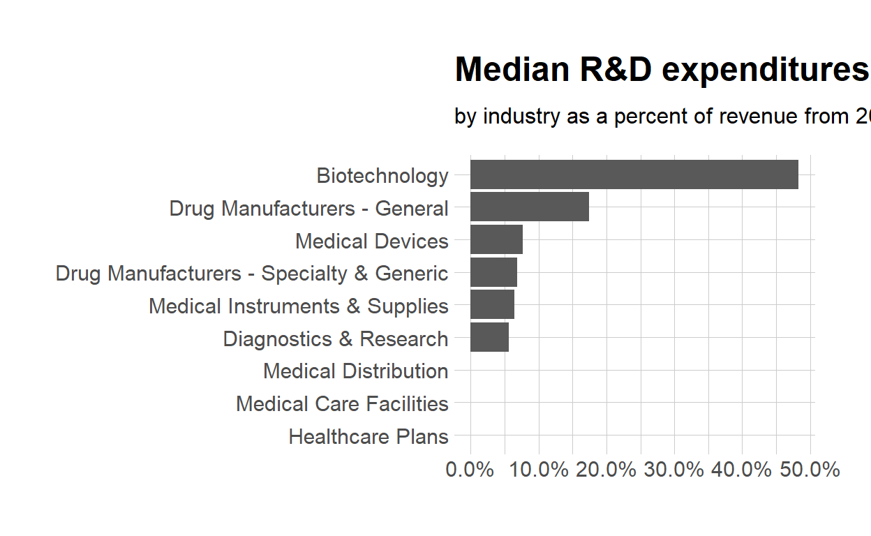
$ med_rnd_rev <dbl> 0.48317287, 0.05620271, 0.17451442, 0.0685187...- Create a static bar chart
-use ggplot to initialize the chart -data is df -the variable industry is mapped to the x-axis -reorder it based the value of med_rnd_rev -the variable med_rnd_revis mapped to the y-axis -add a bar chart using geom_col -use scale_y_continuous to label the y-axis with percent -use coord_flip() to flip the coordinates -use labs to add title, subtitle and remove x and y-axis -use theme_ipsum() from the hrbrthemes package to improve the themes
ggplot(data = df,
       mapping = aes(
       x = reorder(industry, med_rnd_rev),
       y = med_rnd_rev
       ))+
  geom_col()+
  scale_y_continuous(labels = scales::percent)+
  coord_flip()+
  labs(
    title = "Median R&D expenditures" ,
    subtitle = "by industry as a percent of revenue from 2011 to 2018",
    x = NULL, y = NULL) +
  theme_ipsum()
- Save the last plot to preview.png and add to the yaml chunk at the top
ggsave(filename = "preview.png",
       path = here::here("_posts", "2021-03-06-joining-data"))
- Create an interactive bar chart using the package echarts4r
-start with the data df -use arrange to reorder med_rnd_rev -use e_charts to initialize a chart -the variable industry is mapped to the x-axis -add a bar chart using e_bar with the values of med_rnd_rev -use e_flip_coords() to flip the coordinates -use e_title to add the title and the subtitle -use e_legend to remove the legends -use e_x_axis to change format of labels on x-axis to percent -use e_y_axis to remove labels on y-axis- -use e_theme to change the theme. Find more themes here
df  %>%
  arrange(med_rnd_rev)  %>%
  e_charts(
    x = industry
    )  %>%
  e_bar(
    serie = med_rnd_rev,
    name = "median"
    )  %>%
  e_flip_coords()  %>%
  e_tooltip()  %>%
  e_title(
    text = "Median industry R&D expenditures",
    subtext = "by industry as a percent of revenue from 2011 to 2018",
    left = "center") %>%
  e_legend(FALSE) %>%
  e_x_axis(
    formatter = e_axis_formatter("percent", digits = 0)
    )  %>%
  e_y_axis(
    show = FALSE
  )  %>%
  e_theme("infographic")